
# MLAir - Machine Learning on Air Data
MLAir (Machine Learning on Air data) is an environment that simplifies and accelerates the creation of new machine
learning (ML) models for the analysis and forecasting of meteorological and air quality time series. You can find the
docs [here](http://toar.pages.jsc.fz-juelich.de/mlair/docs/).
[[_TOC_]]
# Installation
MLAir is based on several python frameworks. To work properly, you have to install all packages from the
`requirements.txt` file. Additionally to support the geographical plotting part it is required to install geo
packages built for your operating system. Unfortunately, the names of these package may differ for different systems.
In this instruction, we try to address users of different operating systems namely openSUSE Leap, Ubuntu and macOS.
If the installation is still not working, we recommend skipping the geographical plot. We have put together a small
workaround [here](#workaround-to-skip-geographical-plot). For special instructions to install MLAir on the Juelich
HPC systems, see [here](#special-instructions-for-installation-on-jülich-hpc-systems).
* Make sure to have the **python3.6** version installed.
* (geo) A **c++ compiler** is required for the installation of the program **cartopy**
* (geo) Install **proj** and **GEOS** on your machine using the console.
* Install the **python3.6 develop** libraries.
* Install all **requirements** from [`requirements.txt`](https://gitlab.version.fz-juelich.de/toar/mlair/-/blob/master/requirements.txt)
preferably in a virtual environment. You can use `pip install -r requirements.txt` to install all requirements at
once. Note, we recently updated the version of Cartopy and there seems to be an ongoing
[issue](https://github.com/SciTools/cartopy/issues/1552) when installing numpy and Cartopy at the same time. If you
run into trouble, you could use `cat requirements.txt | cut -f1 -d"#" | sed '/^\s*$/d' | xargs -L 1 pip install`
instead.
* Installation of **MLAir**:
* Either clone MLAir from the [gitlab repository](https://gitlab.version.fz-juelich.de/toar/mlair.git)
and use it without installation (beside the requirements)
* or download the distribution file ([current version](https://gitlab.version.fz-juelich.de/toar/mlair/-/blob/master/dist/mlair-1.3.0-py3-none-any.whl))
and install it via `pip install <dist_file>.whl`. In this case, you can simply import MLAir in any python script
inside your virtual environment using `import mlair`.
* (tf) Currently, TensorFlow-1.13 is mentioned in the requirements. We already tested the TensorFlow-1.15 version and couldn't
find any compatibility errors. Please note, that tf-1.13 and 1.15 have two distinct branches each, the default branch
for CPU support, and the "-gpu" branch for GPU support. If the GPU version is installed, MLAir will make use of the GPU
device.
## openSUSE Leap 15.1
* c++ compiler
`sudo zypper install gcc-c++`
* geo packages
`sudo zypper install proj geos-devel`
* depending on the pre-installed packages it could be required to install further packages
`sudo zypper install libproj-devel binutils gdal-devel graphviz graphviz-gnome`
* python develop libraries
`sudo zypper install python3-devel`
## Ubuntu 20.04.1
* c++ compiler
`sudo apt install build-essential`
* geo packages
`sudo apt install proj-bin libgeos-dev libproj-dev`
* depending on the pre-installed packages it could be required to install further packages
`sudo apt install graphviz libgeos++-dev`
* python develop libraries
`sudo apt install python3.6-dev`
## macOS & windows
The installation on macOS is not tested yet. The following commands are possibly needed:
`brew install geos`
`sudo port install graphviz`
The installation on Windows is not tested yet.
# How to start with MLAir
In this section, we show three examples how to work with MLAir. Note, that for these examples MLAir was installed using
the distribution file. In case you are using the git clone it is required to adjust the import path if not directly
executed inside the source directory of MLAir. There is also a downloadable
[Jupyter Notebook](https://gitlab.version.fz-juelich.de/toar/mlair/-/blob/master/supplement/Examples_from_manuscript.ipynb)
provided in that you can run the following examples. Note that this notebook still requires an installation of MLAir.
## Example 1
We start MLAir in a dry run without any modification. Just import mlair and run it.
```python
import mlair
# just give it a dry run without any modification
mlair.run()
```
The logging output will show you many informations. Additional information (including debug messages) are collected
inside the experiment path in the logging folder.
```log
INFO: DefaultWorkflow started
INFO: ExperimentSetup started
INFO: Experiment path is: /home/<usr>/mlair/testrun_network
...
INFO: load data for DEBW107 from JOIN
INFO: load data for DEBY081 from JOIN
INFO: load data for DEBW013 from JOIN
INFO: load data for DEBW076 from JOIN
INFO: load data for DEBW087 from JOIN
...
INFO: Training started
...
INFO: DefaultWorkflow finished after 0:03:04 (hh:mm:ss)
```
## Example 2
Now we update the stations and customise the window history size parameter.
```python
import mlair
# our new stations to use
stations = ['DEBW030', 'DEBW037', 'DEBW031', 'DEBW015', 'DEBW107']
# expanded temporal context to 14 (days, because of default sampling="daily")
window_history_size = 14
# restart the experiment with little customisation
mlair.run(stations=stations,
window_history_size=window_history_size)
```
The output looks similar, but we can see, that the new stations are loaded.
```log
INFO: DefaultWorkflow started
INFO: ExperimentSetup started
...
INFO: load data for DEBW030 from JOIN
INFO: load data for DEBW037 from JOIN
INFO: load data for DEBW031 from JOIN
INFO: load data for DEBW015 from JOIN
...
INFO: Training started
...
INFO: DefaultWorkflow finished after 00:02:03 (hh:mm:ss)
```
## Example 3
Let's just apply our trained model to new data. Therefore we keep the window history size parameter but change the stations.
In the run method, we need to disable the trainable and create new model parameters. MLAir will use the model we have
trained before. Note, this only works if the experiment path has not changed or a suitable trained model is placed
inside the experiment path.
```python
import mlair
# our new stations to use
stations = ['DEBY002', 'DEBY079']
# same setting for window_history_size
window_history_size = 14
# run experiment without training
mlair.run(stations=stations,
window_history_size=window_history_size,
create_new_model=False,
train_model=False)
```
We can see from the terminal that no training was performed. Analysis is now made on the new stations.
```log
INFO: DefaultWorkflow started
...
INFO: No training has started, because train_model parameter was false.
...
INFO: DefaultWorkflow finished after 0:01:27 (hh:mm:ss)
```
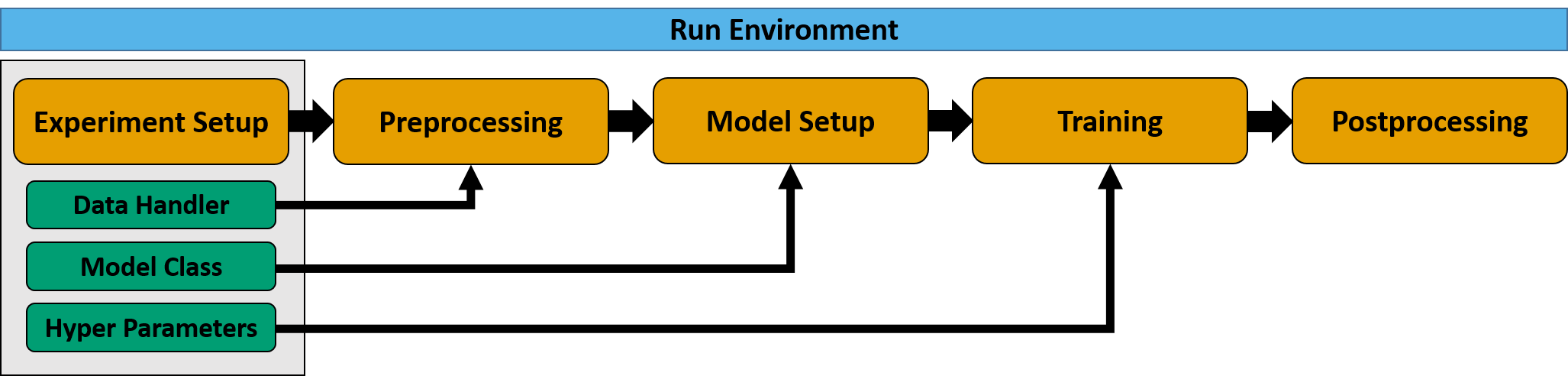
# Default Workflow
MLAir is constituted of so-called `run_modules` which are executed in a distinct order called `workflow`. MLAir
provides a `default_workflow`. This workflow runs the run modules `ExperimentSetup`, `PreProcessing`,
`ModelSetup`, `Training`, and `PostProcessing` one by one.
```python
import mlair
# create your custom MLAir workflow
DefaultWorkflow = mlair.DefaultWorkflow()
# execute default workflow
DefaultWorkflow.run()
```
The output of running this default workflow will be structured like the following.
```log
INFO: DefaultWorkflow started
INFO: ExperimentSetup started
...
INFO: ExperimentSetup finished after 00:00:01 (hh:mm:ss)
INFO: PreProcessing started
...
INFO: PreProcessing finished after 00:00:11 (hh:mm:ss)
INFO: ModelSetup started
...
INFO: ModelSetup finished after 00:00:01 (hh:mm:ss)
INFO: Training started
...
INFO: Training finished after 00:02:15 (hh:mm:ss)
INFO: PostProcessing started
...
INFO: PostProcessing finished after 00:01:37 (hh:mm:ss)
INFO: DefaultWorkflow finished after 00:04:05 (hh:mm:ss)
```
# Customised Run Module and Workflow
It is possible to create new custom run modules. A custom run module is required to inherit from the base class
`RunEnvironment` and to hold the constructor method `__init__()`. This method has to execute the module on call.
In the following example, this is done by using the `_run()` method that is called by the initialiser. It is
possible to parse arguments to the custom run module as shown.
```python
import mlair
import logging
class CustomStage(mlair.RunEnvironment):
"""A custom MLAir stage for demonstration."""
def __init__(self, test_string):
super().__init__() # always call super init method
self._run(test_string) # call a class method
def _run(self, test_string):
logging.info("Just running a custom stage.")
logging.info("test_string = " + test_string)
epochs = self.data_store.get("epochs")
logging.info("epochs = " + str(epochs))
```
If a custom run module is defined, it is required to adjust the workflow. For this, you need to load the empty
`Workflow` class and add each run module that is required. The order of adding modules defines the order of
execution if running the workflow.
```python
# create your custom MLAir workflow
CustomWorkflow = mlair.Workflow()
# provide stages without initialisation
CustomWorkflow.add(mlair.ExperimentSetup, epochs=128)
# add also keyword arguments for a specific stage
CustomWorkflow.add(CustomStage, test_string="Hello World")
# finally execute custom workflow in order of adding
CustomWorkflow.run()
```
The output will look like:
```log
INFO: Workflow started
...
INFO: ExperimentSetup finished after 00:00:12 (hh:mm:ss)
INFO: CustomStage started
INFO: Just running a custom stage.
INFO: test_string = Hello World
INFO: epochs = 128
INFO: CustomStage finished after 00:00:01 (hh:mm:ss)
INFO: Workflow finished after 00:00:13 (hh:mm:ss)
```
# Custom Model
Create your own model to run your personal experiment. To guarantee a proper integration in the MLAir workflow, models
are restricted to inherit from the `AbstractModelClass`. This will ensure a smooth training and evaluation
behaviour.
## How to create a customised model?
* Create a new model class inheriting from `AbstractModelClass`
```python
from mlair import AbstractModelClass
class MyCustomisedModel(AbstractModelClass):
def __init__(self, input_shape: list, output_shape: list):
# set attributes shape_inputs and shape_outputs
super().__init__(input_shape[0], output_shape[0])
# apply to model
self.set_model()
self.set_compile_options()
self.set_custom_objects(loss=self.compile_options['loss'])
```
* Make sure to add the `super().__init__()` and at least `set_model()` and `set_compile_options()` to your
custom init method.
* The shown model expects a single input and output branch provided in a list. Therefore shapes of input and output are
extracted and then provided to the super class initialiser.
* Some general settings like the dropout rate are set in the init method additionally.
* If you have custom objects in your model, that are not part of the keras or tensorflow frameworks, you need to add
them to custom objects. To do this, call `set_custom_objects` with arbitrarily kwargs. In the shown example, the
loss has been added for demonstration only, because we use a build-in loss function. Nonetheless, we always encourage
you to add the loss as custom object, to prevent potential errors when loading an already created model instead of
training a new one.
* Now build your model inside `set_model()` by using the instance attributes `self._input_shape` and
`self._output_shape` and storing the model as `self.model`.
```python
import keras
from keras.layers import PReLU, Input, Conv2D, Flatten, Dropout, Dense
class MyCustomisedModel(AbstractModelClass):
def set_model(self):
x_input = Input(shape=self._input_shape)
x_in = Conv2D(4, (1, 1))(x_input)
x_in = PReLU()(x_in)
x_in = Flatten()(x_in)
x_in = Dropout(0.1)(x_in)
x_in = Dense(16)(x_in)
x_in = PReLU()(x_in)
x_in = Dense(self._output_shape)(x_in)
out = PReLU()(x_in)
self.model = keras.Model(inputs=x_input, outputs=[out])
```
* Your are free how to design your model. Just make sure to save it in the class attribute model.
* Additionally, set your custom compile options including the loss definition.
```python
from keras.losses import mean_squared_error as mse
class MyCustomisedModel(AbstractModelClass):
def set_compile_options(self):
self.initial_lr = 1e-2
self.optimizer = keras.optimizers.SGD(lr=self.initial_lr, momentum=0.9)
self.loss = mse
self.compile_options = {"metrics": ["mse", "mae"]}
```
* The allocation of the instance parameters `initial_lr`, `optimizer`, and `lr_decay` could be also part of
the model class' initialiser. The same applies to `self.loss` and `compile_options`, but we recommend to use
the `set_compile_options` method for the definition of parameters, that are related to the compile options.
* More important is that the compile options are actually saved. There are three ways to achieve this.
* (1): Set all compile options by parsing a dictionary with all options to `self.compile_options`.
* (2): Set all compile options as instance attributes. MLAir will search for these attributes and store them.
* (3): Define your compile options partly as dictionary and instance attributes (as shown in this example).
* If using (3) and defining the same compile option with different values, MLAir will raise an error.
Incorrect: (Will raise an error because of a mismatch for the `optimizer` parameter.)
```python
def set_compile_options(self):
self.optimizer = keras.optimizers.SGD()
self.loss = keras.losses.mean_squared_error
self.compile_options = {"optimizer" = keras.optimizers.Adam()}
```
## How to plug in the customised model into the workflow?
* Make use of the `model` argument and pass `MyCustomisedModel` when instantiating a workflow.
```python
from mlair.workflows import DefaultWorkflow
workflow = DefaultWorkflow(model=MyCustomisedModel)
workflow.run()
```
## Specials for Branched Models
* If you have a branched model with multiple outputs, you need either set only a single loss for all branch outputs or
provide the same number of loss functions considering the right order.
```python
class MyCustomisedModel(AbstractModelClass):
def set_model(self):
...
self.model = keras.Model(inputs=x_input, outputs=[out_minor_1, out_minor_2, out_main])
def set_compile_options(self):
self.loss = [keras.losses.mean_absolute_error] + # for out_minor_1
[keras.losses.mean_squared_error] + # for out_minor_2
[keras.losses.mean_squared_error] # for out_main
```
## How to access my customised model?
If the customised model is created, you can easily access the model with
```python
>>> MyCustomisedModel().model
<your custom model>
```
The loss is accessible via
```python
>>> MyCustomisedModel().loss
<your custom loss>
```
You can treat the instance of your model as instance but also as the model itself. If you call a method, that refers to
the model instead of the model instance, you can directly apply the command on the instance instead of adding the model
parameter call.
```python
>>> MyCustomisedModel().model.compile(**kwargs) == MyCustomisedModel().compile(**kwargs)
True
```
# Data Handlers
Data handlers are responsible for all tasks related to data like data acquisition, preparation and provision. A data
handler must inherit from the abstract base class `AbstractDataHandler` and requires the implementation of the
`__init__()` method and the accessors `get_X()` and `get_Y()`. In the following, we show an example how a custom data
handler could look like.
```python
import datetime as dt
import numpy as np
import pandas as pd
import xarray as xr
from mlair.data_handler import AbstractDataHandler
class DummyDataHandler(AbstractDataHandler):
def __init__(self, name, number_of_samples=None):
"""This data handler takes a name argument and the number of samples to generate. If not provided, a random
number between 100 and 150 is set."""
super().__init__()
self.name = name
self.number_of_samples = number_of_samples if number_of_samples is not None else np.random.randint(100, 150)
self._X = self.create_X()
self._Y = self.create_Y()
def create_X(self):
"""Inputs are random numbers between 0 and 10 with shape (no_samples, window=14, variables=5)."""
X = np.random.randint(0, 10, size=(self.number_of_samples, 14, 5)) # samples, window, variables
datelist = pd.date_range(dt.datetime.today().date(), periods=self.number_of_samples, freq="H").tolist()
return xr.DataArray(X, dims=['datetime', 'window', 'variables'], coords={"datetime": datelist,
"window": range(14),
"variables": range(5)})
def create_Y(self):
"""Targets are normal distributed random numbers with shape (no_samples, window=5, variables=1)."""
Y = np.round(0.5 * np.random.randn(self.number_of_samples, 5, 1), 1) # samples, window, variables
datelist = pd.date_range(dt.datetime.today().date(), periods=self.number_of_samples, freq="H").tolist()
return xr.DataArray(Y, dims=['datetime', 'window', 'variables'], coords={"datetime": datelist,
"window": range(5),
"variables": range(1)})
def get_X(self, upsampling=False, as_numpy=False):
"""Upsampling parameter is not used for X."""
return np.copy(self._X) if as_numpy is True else self._X
def get_Y(self, upsampling=False, as_numpy=False):
"""Upsampling parameter is not used for Y."""
return np.copy(self._Y) if as_numpy is True else self._Y
def __str__(self):
return self.name
```
# Special Remarks
## Workaround to skip geographical plot
If it is not possible to install all required geo libraries on your system, a good compromise is to skip the creation
of the geographical plot. Therefore, it is required to remove the plot from the `plot_list` manually. We recommend to
use this code snippet as a starting point.
```python
from mlair.helpers import remove_items
from mlair.configuration.defaults import DEFAULT_PLOT_LIST
mlair.run(plot_list=remove_items(DEFAULT_PLOT_LIST, "PlotStationMap"))
```
## Special instructions for installation on Jülich HPC systems
_Please note, that the HPC setup is customised for JUWELS and HDFML. When using another HPC system, you can use the HPC
setup files as a skeleton and customise it to your needs._
The following instruction guide you through the installation on JUWELS and HDFML.
* Clone the repo to HPC system (we recommend to place it in `/p/projects/<project name>`).
* Setup venv by executing `source setupHPC.sh`. This script loads all pre-installed modules and creates a venv for
all other packages. Furthermore, it creates slurm/batch scripts to execute code on compute nodes.
You have to enter the HPC project's budget name (--account flag).
* The default external data path on JUWELS and HDFML is set to `/p/project/deepacf/intelliaq/<user>/DATA/toar_<sampling>`.
To choose a different location open `run.py` and add the following keyword argument to `ExperimentSetup`:
`data_path=<your>/<custom>/<path>`.
* Execute `python run.py` on a login node to download example data. The program will throw an OSerror after downloading.
* Execute either `sbatch run_juwels_develgpus.bash` or `sbatch run_hdfml_batch.bash` to verify that the setup went well.
* Currently cartopy is not working on our HPC system, therefore PlotStations does not create any output.
Note: The method `PartitionCheck` currently only checks if the hostname starts with `ju` or `hdfmll`.
Therefore, it might be necessary to adopt the `if` statement in `PartitionCheck._run`.
## Security using JOIN
* To use hourly data from ToarDB via JOIN interface, a private token is required. Request your personal access token and
add it to `src/join_settings.py` in the hourly data section. Replace the `TOAR_SERVICE_URL` and the `Authorization`
value. To make sure, that this **sensitive** data is not uploaded to the remote server, use the following command to
prevent git from tracking this file: `git update-index --assume-unchanged src/join_settings.py`